Quantum Behavior
(From Richard Feynman’s Lectures on Physics)
1-1 Atomic mechanics
1-2 An experiment with bullets
1-3 An experiment with waves
1-4 An experiment with electrons
1-5 The interference of electron
waves
1-6 Watching the electrons
1-7 First principles of quantum
mechanics
1-8 The uncertainty principle
Note: This chapter is almost exactly
the same as Chapter 37 of Volume I.
1-1 Atomic mechanics
"Quantum mechanics" is the description of the behavior of matter and light
in all its details and, in particular, of the happenings on an atomic scale. Things
on a very small scale behave like nothing that you have any direct experience
about. They do not behave like waves, they do not behave like particles, they do
not behave like clouds, or billiard balls, or weights on springs, or like anything
that you have ever seen.
Newton thought that light was made up of particles, but then it was discovered
that it behaves like a wave. Later, however (in the beginning of the twentieth
century), it was found that light did indeed sometimes behave like a particle.
Historically, the electron, for example, was thought to behave like a particle, and
then it was found that in many respects it behaved like a wave. So it really behaves
like neither. Now we have given up. We say: "It is like neither."
There is one lucky break, however—electrons behave just like light. The
quantum behavior of atomic objects (electrons, protons, neutrons, photons, and
so on) is the same for all, they are all "particle waves," or whatever you want to
call them. So what we learn about the properties of electrons (which we shall use
for our examples) will apply also to all "particles," including photons of light.
The gradual accumulation of information about atomic and small-scale be-
havior during the first quarter of this century, which gave some indications about
how small things do behave, produced an increasing confusion which was finally
resolved in 1926 and 1927 by Schrodinger, Heisenberg, and Born. They finally
obtained a consistent description of the behavior of matter on a small scale. We
take up the main features of that description in this chapter.
Because atomic behavior is so unlike ordinary experience, it is very difficult
to get used to, and it appears peculiar and mysterious to everyone—both to the
novice and to the experienced physicist. Even the experts do not understand it
the way they would like to, and it is perfectly reasonable that they should not,
because all of direct, human experience and of human intuition applies to large
objects. We know how large objects will act, but things on a small scale just do
not act that way. So we have to learn about them in a sort of abstract or imagi-
native fashion and not by connection with our direct experience.
In this chapter we shall tackle immediately the basic element of the mysterious
behavior in its most strange form. We choose to examine a phenomenon which is
impossible, absolutely impossible, to explain in any classical way, and which has
in it the heart of quantum mechanics. In reality, it contains the only mystery.
We cannot make the mystery go away by "explaining" how it works. We will just
re//you how it works. In telling you how it works we will have told you about the
basic peculiarities of all quantum mechanics.
1-2 An experiment with bullets
To try to understand the quantum behavior of electrons, we shall compare
and contrast their behavior, in a particular experimental setup, with the more
familiar behavior of particles like bullets, and with the behavior of waves like
water waves. We consider first the behavior of bullets in the experimental setup
shown diagranimatically in Fig. 1-1. We have a machine gun that shoots a stream
of bullets. It is not a very good gun, in that it sprays the bullets (randomly) over a
fairly large angular spread, as indicated in the figure. In front of the gun we have
l-l
a wall (made of armor plate) that has in it two holes just about big enough to let a
bullet through. Beyond the wall is a backstop (say a thick wall of wood) which will
"absorb" the bullets when they hit it. In front of the wall we have an object which
we shall call a "detector" of bullets. It might be a box containing sand. Any bullet
that enters the detector will be stopped and accumulated. When we wish, we can
empty the box and count the number of bullets that have been caught. The
detector can be moved back and forth (in what we will call the A-direction). With
this apparatus, we can find out experimentally the answer to the question: "What
is the probability that a bullet which passes through the holes in (he wall will
arrive at the backstop at the distance x from the center?" First, you should
realize that we should talk about probability, because we cannot say definitely
where any particular bullet will go. A bullet which happens to hit one of the holes
may bounce off the edges of the hole, and may end up anywhere at all. By "prob-
ability" we mean the chance that the bullet will arrive at the detector, which we can
measure by counting the number which arrive at the detector in a certain time and
then taking the ratio of this number to the total number that hit the backstop during
that time. Or, if we assume that the gun always shoots at the same rate during the
measurements, the probability we want is just proportional to the number that
reach the detector in some standard time interval.
For our present purposes we would like to imagine a somewhat idealized
experiment in which the bullets are not real bullets, but are indestructible bullets—
they cannot break in half. In our experiment we find that bullets always arrive in
lumps, and when we find something in the detector, it is always one whole bullet.
If the rate at which the machine gun fires is made very low, we find that at any given
moment either nothing arrives, or one and only one—exactly one—bullet arrives
at the backstop. Also, the size of the lump certainly does not depend on the rate
of firing of the gun. We shall say: "Bullets always arrive in identical lumps." What
we measure with our detector is the probability of arrival of a lump. And we meas-
ure the probability as a function of x. The result of such measurements with this
apparatus (we have not yet done the experiment, so we are really imagining the
result) are plotted in the graph drawn in part (c) of Fig. 1-1. In the graph we plot
the probability to the right and x vertically, so that the x-scale fits the diagram of
the apparatus. We call the probability P12 because the bullets may have come
either through hole 1 or through hole 2. You will not be surprised that P12 is
large mear the middle of the graph but gets small if x is very large. You may
wonder, however, why P12 has its maximum value at x = 0. We can understand
this fact if we do our experiment again after covering up hole 2, and once more
while covering up hole 1. When hole 2 is covered, bullets can pass only through
hole 1, and we get the curve marked Pt in part (b) of the figure. As you would
expect, the maximum of P1 occurs at the value of x which is on a straight line with
the gun and hole 1. When hole 1 is closed, we get the symmetric curve P2 drawn
in the figure. P2 is the probability distribution for bullets that pass through hole
2. Comparing parts (b) and (c) of Fig. 1-1, we find the important result that
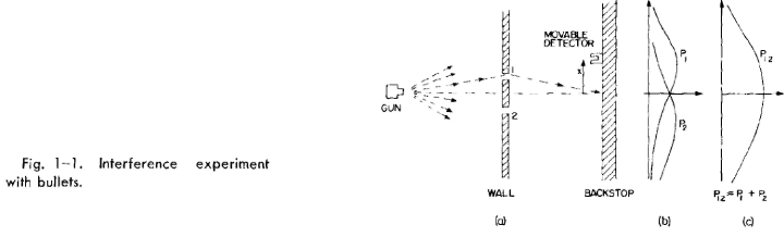
P12= P1 + P2-
(1.1)
1-2
The probabilities just add together. The effect with both holes open is the sum of
the effects with each hole open alone. We shall call this result an observation of
"no interference" for a reason that you will see later. So much for bullets. They
come in lumps, and their probability of arrival shows no interference.
1-3 An experiment with waves
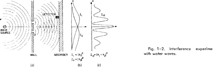
Now we wish to consider an experiment with water waves. The apparatus is
shown diagrarnmatically in Fig. 1-2. We have a shallow trough of water. A small
object labeled the "wave source" is jiggled up and down by a motor and makes
circular waves. To the right of the source we have again a wall with two holes,
and beyond that is a second wall, which, to keep things simple, is an "absorber,"
so that there is no reflection of the waves that arrive there. This can be done by
building a gradual sand "beach." In front of the beach we place a detector which
can he moved back and forth in the x-direction, as before. The detector is now a
device which measures the "intensity" of the wave motion. You can imagine a
gadget which measures the height of the wave motion, but whose scale is calibrated
in proportion to the square of the actual height, so that the reading is proportional
to the intensity of the wave. Our detector reads, then, in proportion to the energy
being carried by the wave—or rather, the rate at which energy is carried to the
detector.
With our wave apparatus, the first thing to notice is that the intensity can
have any size. If the source just moves a very small amount, then there is just a
little bit of wave motion at the detector. When there is more motion at the source,
there is more intensity at the detector. The intensity of the wave can have any
value at all. We would not say that there was any "lumpiness" in the wave intensity.
Now let us measure the wave intensity for various values of x (keeping the
wave source operating always in the same way). We get the interesting-looking
curve marked I12 in part (c) of the figure.
We have already worked out how such patterns can come about when we
studied the interference of electric waves in Volume I. In this case we would
observe that the original wave is diffracted at the holes, and new circular waves
spread out from each hole. If we cover one hole at a time and measure the intensity
distribution at the absorber we find the rather simple intensity curves shown in part
(b) of the figure. I1 is the intensity of the wave from hole 1 (which we find by
measuring when hole 2 is blocked off) and I2 is the intensity of the wave from hole
2 (seen when hole 1 is blocked).
The intensity I12 observed when both holes are open is certainly not the sum
of I1 and I2. We say that there is "interference" of the two waves. At some places
(where the curve I12 has its maxima) the waves are "in phase" and the wave
peaks add together to give a large amplitude and, therefore, a large intensity. We
say that the two waves are "interfering constructively" at such places. There will
be such constructive interference wherever the distance from the detector to one
hole is a whole number of wavelengths larger (or shorter) than the distance from
the detector to the other hole.
1-3
At those places where the two waves arrive at the detector with a phase differ-
ence of pi (where they are "out of phase") the resulting wave motion at the detector
will be the difference of the two amplitudes. The waves "interfere destructively,"
and we get a low value for the wave intensity. We expect such low values wherever
the distance between hole 1 and the detector is different from the distance between
hole 2 and the detector by an odd number of half-wavelengths. The low values of
I12 in Fig. 1-2 correspond to the places where the two waves interfere destructively.
You will remember that the quantitative relationship between I1,, I2, and I12
can be expressed in the following way: The instantaneous height of the water wave
at the detector for the wave from hole 1 can be written as (the real part of)
where the "amplitude" A, is, in general, a complex number. The intensity is
proportional to the mean squared height or. when we use the complex numbers,
to the absolute value squared . Similarly, for hole 2 the height is
 and the
intensity is proportional to When both holes are open, the wave heights
add to give the height and the intensity
 Omitting the
constant of proportionality for our present purposes, the proper relations for
interfering waves are

You will notice that the result is quite different from that obtained with bullets
(Eq. 1-1). If we expand we see that

where 5 is the phase difference between hA and h2- In terms of the intensities, we
could write
The last term in (1.4) is the "interference term." So much for water waves. The
intensity can have any value, and it shows interference.
1-4 An experiment with electrons
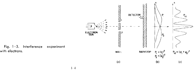
Now we imagine a similar experiment with electrons. It is shown diagram-
matically in Fig. 1-3. We make an electron gun which consists of a tungsten wire
heated by an electric current and surrounded by a metal box with a hole in it. If
the wire is at a negative voltage with respect to the box, electrons emitted by the
wire will be accelerated toward the walls and some will pass through the hole.
All the electrons which come out of the gun will have (nearly) the same energy.
In front of the gun is again a wall (just a thin metal plate) with two holes in it.
Beyond the wall is another plate which will serve as a "backstop." In front of the
backstop we place a movable detector. The detector might be a geiger counter or,
perhaps better, an electron multiplier, which is connected to a loudspeaker.
We should say right away that you should not try to set up this experiment
(as you could have done with the two we have already desci ihed). This experiment
has never been done in just this way. The trouble is that the apparatus would have
to be made on an impossibly small scale to show the effects we are interested in.
We are doing a "thought experiment," which we have chosen because it is easy to
think about. We know the results that would be obtained because there are many
experiments that have been done, in which the scale and the proportions have
been chosen to show the effects we shall describe.
The first thing we notice with our electron experiment is that we hear sharp
"clicks" from the detector (that is, from the loudspeaker). And all "clicks" are
the same. There are no "half-clicks."
We would also notice that the "clicks" come very erratically. Something like:
click.....click-click . . . click........click .... click-click......click . . . ,
etc., just as you have, no doubt, heard a geiger counter operating. If we count
the clicks which arrive in a sufficiently long time—say for many minutes- and
then count again for another equal period, we find that the two numbers are very
nearly the same. So we can speak of the average rate at which the clicks are heard
(so-and-so-many clicks per minute on the average).
As we move the detector around, the rate at which the clicks appear is faster
or slower, but the size (loudness) of each click is always the same. If we lower the
temperature of the wire in the gun, the rate of clicking slows down, but still each
click sounds the same. We would notice also that if we put two separate detectors
at the backstop, one or the other would click, but never both at once. (Except that
once in a while, if there were two clicks very close together in time, our ear might
not sense the separation.) We conclude, therefore, that whatever arrives at the
backstop arrives in "lumps." All the "lumps" are the same size: only whole
"lumps" arrive, and they arrive one at a time at the backstop. Wc shall say:
"Electrons always arrive in identical lumps."
Just as for our experiment with bullets, we can now proceed to find experi-
mentally the answer to the question: "What is the relative probability that an
electron 'lump' will arrive at the backstop at various distances x from the center?"
As before, we obtain the relative probability by observing the rate of clicks, holding
the operation of the gun constant. The probability that lumps will arrive at a
particular x is proportional to the average rate of clicks at that x.
The result of our experiment is the interesting curve marked P12 in part (c)
of Fig. 1-3. Yes! That is the way electrons go.
1-5 The interference of electron waves
Now let us try to analyze the curve of Fig. 1-3 to sec whether we can under-
stand the behavior of the electrons. The first thing we would say is that since they
come in lumps, each lump, which we may as well call an electron, has come either
through hole 1 or through hole 2. Let us write this in the form of a "Proposition":
Proposition A: Each electron either goes through hole 1 or it goes through
hole 2.
Assuming Propositon A, all electrons that arrive at the backstop can be di-
vided into two classes: (I) those that come through hole 1, and (2) those that come
through hole 2. So our observed curve must be the sum of the effects of the elec-
trons which come through hole 1 and the electrons which come through hole 2.
Let us check this idea by experiment. First, we will make a measurement for those
electrons that come through hole 1. We block off hole 2 and make our counts of
the clicks from the detector. From the clicking rate, we get P1. The result of the
measurement is shown by the curve marked P1 in part (b) of Fig. 1-3. The result
seems quite reasonable. In a similar way, we measure P2, the probability distribu-
tion for the electrons that come through hole 2. The result of this measurement
is also drawn in the figure.
The result P12 obtained with both holes open is clearly not the sum of P1 and
P2, the probabilities for each hole alone. In analogy with our water-wave experi-
1-5
ment, we say: "There is interference."
 (1.5)
(1.5)
How can such an interference come about? Perhaps we should say: "Well,
that means, presumably, that it is not true that the lumps go either through hole
1 or hole 2, because if they did, the probabilities should add. Perhaps they go in a
more complicated way. They split in half and . . " But no! They cannot, they
always arrive in lumps . . . "Well, perhaps some of them go through I, and then
they go around through 2, and then around a few more times, or by some other
complicated path . then by closing hole 2, we changed the chance that an elec-
tron that started out through hole 1 would finally get to the backstop " But
notice! There are some points at which very few electrons arrive when both holes
are open, but which receive many electrons if we close one hole, so closing one
hole increased the number from the other. Notice, however, that at the center
of the pattern, P12 is more than twice as large as P1 + P2. It is as though closing
one hole decreased the number of electrons which come through the other hole.
It seems hard to explain both effects by proposing that the electrons travel in
complicated paths.
It is all quite mysterious. And the more you look at it the more mysterious
it seems. Many ideas have been concocted to try to explain the curve for P12 in
terms of individual electrons going around in complicated ways through the holes.
None of them has succeeded. None of them can get the right curve for P12 in
terms of P1 and P2.
Yet, surprisingly enough, the mathematics for relating P1 and P2 to P12
is extremely simple. For P12 is just like the curve I12 of Fig. 1-2, and that was
simple. What is going on at the backstop can be described by two complex numbers
that we can call and
and (they are functions of x, of course). The absolute square
of  gives the effect with only hole 1 open. That is, P1=
 The effect with
only hole 2 open is given by in the same way. That is. P2 =
  And the
combined effect of the two holes is just Pl2 =  The mathematics
is the same as that we had for the water waves! (It is hard to see how one could
get such a simple result from a complicated game of electrons going back and forth
through the plate on some strange trajectory.)
We conclude the following: The electrons arrive in lumps, like particles, and
the probability of arrival of these lumps is distributed like the distribution of
intensity of a wave. It is in this sense that an electron behaves "sometimes like a
particle and sometimes like a wave."
Incidentally, when we were dealing with classical waves we defined the in-
tensity as the mean over time of the square of the wave amplitude, and we used
complex numbers as a mathematical trick to simplify the analysis. But in quantum
mechanics it turns out that the amplitudes must be represented by complex num-
bers. The real parts alone will not do. That is a technical point, for the moment,
because the formulas look just the same.
Since the probability of arrival through both holes is given so simply, although
it is not equal to (P1 + P2 ), that is really all there is to say. But there are a large
number of subtleties involved in the fact that nature does work this way. Wc
would like to illustrate some of these subtleties for you now. First, since the num-
ber that arrives at a particular point is not equal to the number that arrives through
1 plus the number that arrives through 2, as we would have concluded from
Proposition A, undoubtedly we should conclude that Proposition A is false. It is
not true that the electrons go either through hole 1 or hole 2. But that conclusion
can be tested by another experiment.
1-6 Watching the electrons
We shall now try the following experiment. To our electron apparatus we
add a very strong light source, placed behind the wall and between the two holes,
as shown in Fig. 1-4. We know that electric charges scatter light. So when an
1-6
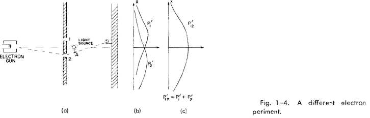
electron passes, however it does pass, on its way to the detector, it will scatter some
light to our eye. and we can see where the electron goes. If, for instance, an electron
were to take the path via hole 2 that is sketched in Fig. 1-4, we should see a flash
of light coming from the vicinity of the place marked A in the figure. If an electron
passes through hole 1, we would expect to see a flash from the vicinity of the upper
hole. If it should happen that we get light from both places at the same time,
because the electron divides in half . . . Let us just do the experiment!
Here is what we see: every time that we hear a "click" from our electron de-
tector (at the backstop), we also see a flash of light either near hole I or near hole
2, but never both at once! And we observe the same result no matter where we put
the detector. From this observation we conclude that when we look at the electrons
we find that the electrons go either through one hole or the other. Experimentally,
Proposition A is necessarily true.
What, then, is wrong with our argument against Proposition A? Why isn't
P12 just equal to P1 + P2. Back to experiment! Let us keep track of the electrons
and find out what they are doing. For each position (x-location) of the detector
we will count the electrons that arrive and also keep track of which hole they went
through, by watching for the flashes. We can keep track of things this way:
whenever wc hear a "click" we will put a count in Column 1 if we see the flash near
hole 1, and if we see the flash near hole 2, we will record a count in Column 2.
Every electron which arrives is recorded in one of two classes: those which come
through 1 and those which come through 2. From the number recorded in Column
1 we get the probability P1' that an electron will arrive at the detector via hole 1;
and from the number recorded in Column 2 we get P2' , the probability that an
electron will arrive at the detector via hole 2. If we now repeat such a measurement
for many values of x, we get the curves for P1' and P2' shown in part (b) of Fig, 1-4.
Well, that is not too surprising! We get for P1' something quite similar to
what we got before for P1 by blocking off hole 2; and P2' is similar to what we got
by blocking hole 1. So there is not any complicated business like going through
both holes. When we watch them, the electrons come through just as we would
expect them to come through. Whether the holes are closed or open, those which
we see come through hole 1 are distributed in the same way whether hole 2 is open
or closed.
But wait! What do we have now for the total probability, the probability that
an electron will arrive at the detector by any route? We already have that informa-
tion. We just pretend that we never looked at the light flashes, and we lump to-
gether the detector clicks which we have separated into the two columns. We
must just add the numbers. For the probability that an electron will arrive at the
backstop by passing through either hole, we do find P12' = P1 + P2. That is,
although we succeeded in watching which hole our electrons come through, we
no longer get the old interference curve P12, but a new one, P12', showing no
interference! If we turn out the light P12 is restored.
Wc must conclude that when we look at the electrons the distribution of them
on the screen is different than when we do not look. Perhaps it is turning on our
light source that disturbs things? It must be that the electrons are very delicate,
and the light, when it scatters off the electrons, gives them a jolt that changes their
1-7
motion. We know that the electric field of the light acting on a charge will exert
a force on it. So perhaps we should expect the motion to be changed. An>way,
the light exerts a big influence on the electrons. By trying to "watch" the electrons
we have changed their motions. That is, the jolt given to the electron when the
photon is scattered by it is such as to change the electron's motion enough so that
if it might have gone to where P12 was at a maximum it will instead land where
P12 was a minimum; that is why we no longer see the wavy interference effects.
You may be thinking: "Don't use such a bright source! Turn the brightness
down! The light waves will then be weaker and will not disturb the electrons so
much. Surely, by making the light dimmer and dimmer, eventually the wave
will be weak enough that it will have a negligible effect." O.K. Let's try it. The
first thing we observe is that the flashes of light scattered from the electrons as
they pass by does not get weaker. // is always the same-sized flash. The only thing
that happens as the light is made dimmer is that sometimes we hear a "click"
from the detector but see no flash at all. The electron has gone by without being
"seen." What we are observing is that light also acts like electrons, we knew that
it was "wavy," but now we find that it is also "lumpy." It always arrives—or is
scattered—in lumps that we call "photons." As we turn down the intensity of
the light source we do not change the size of the photons, only the rate at which
they are emitted. That explains why, when our source is dim, some electrons get
by without being seen. There did not happen to be a photon around at the time
the electron went through.
This is all a little discouraging. If it is true that whenever we "see" the electron
we see the same-sized flash, then those elections we see are always the disturbed
ones. Let us try the experiment with a dim light anyway. Now whenever we hear
a click in the detector we will keep a count in three columns: in Column (I) those
electrons seen by hole 1, in Column (2) those electrons seen by hole 2, and in
Column (3) those electrons not seen at all. When we work up our data (computing
the probabilities) we find these results: Those "seen by hole 1" have a distribution
like P1'; those "seen by hole 2'" have a distiibution like P2' (so that those "seen by
either hole 1 or 2" have a distribution like P12'); and those "not seen at all" have a
"wavy" distribution just like P12 of Fig. 1-3! //' the electrons are not seen, we
have interference1.
That is understandable. When we do not see the electron, no photon disturbs
it, and when we do see it, a photon has disturbed it. There is always the same
amount of disturbance because the light photons all produce the same-sized effects
and the effect of the photons being scattered is enough to smear out any inter-
ference effect.
Is there not some way we can see the electrons without disturbing them?
We learned in an earlier chapter that the momentum carried by a "photon"
is inversely proportional to its wavelength (p = h / lambda). Certainly the jolt given
to the electron when the photon is scattered toward our eye depends on the
momentum that photon carries. Aha! If we want to disturb the electrons only
slightly we should not have lowered the intensity of the light, we should have
lowered its frequency (the same as increasing its wavelength). Let us use light of
a redder color. We could even use infrared light, or radiowaves (like radar), and
"see" where the electron went with the help of some equipment that can "see"
light of these longer wavelengths. If we use "gentler" light perhaps we can avoid
disturbing the electrons so much.
Let us try the experiment with longer waves. We shall keep repeating our ex-
periment, each time with light of a longer wavelength. At first, nothing seems to
change. The results are the same. Then a terrible thing happens. You remember
that when we discussed the microscope we pointed out that, due to the wave nature
of the light, there is a limitation on how close two spots can be and still be seen
as two separate spots. This distance is of the order of the wavelength of light. So
now, when we make the wavelength longer than the distance between our holes,
we see a big fuzzy flash when the light is scattered by the electrons. We can no
longer tell which hole the electron went through! We just know it went somewhere!
And it is just with light of this color that we find that the jolts given to the electron
1-8
are small enough so that P12' begins to look like P12—that we begin to get some
interference effect. And it is only for wavelengths much longer than the separation
of the two holes (when we have no chance at all of telling where the electron went)
that the disturbance due to the light gets sufficiently small that we again get the
curve P12 shown in Fig. 1-3.
In our experiment we find that it is impossible to arrange the light in such a
way lhat one can tell which hole the electron went through, and at the same time
not disturb the pattern. It was suggested by Heisenberg that (he then new laws of
nature could only be consistent if there were some basic limitation on our experi-
mental capabilities not previously recognized. He proposed, as a general principle,
his uncertainty principle, which we can state in terms of our experiment as follows:
"It is impossible to design an apparatus to determine which hole the electron passes
through, that will not at the same time disturb the electrons enough to destroy the
interference pattern." If an apparatus is capable of determining which hole the
electron goes through, it cannot be so delicate that it does not disturb the pattern in
an essential way. No one has ever found (or even thought of) a way around the
uncertainty principle. So we must assume that it describes a basic characteristic
of nature.
The complete theory of quantum mechanics which we now use to describe
atoms and, in fact, all matter, depends on the correctness of the uncertainty prin-
ciple. Since quantum mechanics is such a successful theory, our belief in the
uncertainty principle is reinforced. But if a way to "beat" the uncertainty principle
were ever discovered, quantum mechanics would give inconsistent results and
would have to be discarded as a valid theory of nature.
"Well," you say, "what about Proposition A? Is it true, or is it not true,
that the electron either goes through hole 1 or it goes through hole 2?" The only
answer that can be given is that we have found from experiment that there is a
certain special way that we have to think in order that we do not get into incon-
sistencies. What we must say (to avoid making wrong predictions) is the following.
If one looks at the holes or, more accurately, if one has a piece of apparatus which
is capable of determining whether the electrons go through hole 1 or hole 2, then
one can say that it goes either through hole 1 or hole 2. But, when one does not
try to tell which way the electron goes, when there is nothing in the experiment to
disturb the electrons, then one may not say that an electron goes either through
hole 1 or hole 2. If one docs say that, and starts to make any deductions from the
statement, he will make errors in the analysis. This is the logical tightrope on
which we must walk if we wish to describe nature successfully.
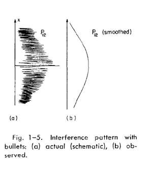
If the motion of all matter—as well as electrons—must be described in terms
of waves, what about the bullets in our first experiment? Why didn't we see an
interference pattern there? It turns out that for the bullets the wavelengths were so
tiny that the interference patterns became very fine. So fine, in fact, that with any
detector of finite size one could not distinguish the separate maxima and minima.
What we saw was only a kind of average, which is the classical curve. In Fig. 1-5
we have tried to indicate schematically what happens with large-scale objects.
Part (a) of the figure shows the probability distribution one might predict for
bullets, using quantum mechanics. The rapid wiggles are supposed to represent
the interference pattern one gets for waves of very short wavelength. Any physical
detector, however, straddles several wiggles of the probability curve, so that the
measurements show the smooth curve drawn in part (b) of the figure.
1-7 First principles of quantum mechanics
We will now write a summary of the main conclusions of our experiments.
We will, however, put the results in a form which makes them true for a general
class of such experiments. We can write our summary more simply if we first
define an "ideal experiment" as one in which there are no uncertain external
influences, i.e., no jiggling or other things going on that we cannot take into ac-
1-9
count. We would be quite precise if we said: "An ideal experiment is one in which
all of the initial and final conditions of the experiment are completely specified."
What we will call "an event" is, in general, just a specific set of initial and final
conditions. (For example: "an electron leaves the gun, arrives at the detector, and
nothing else happens.") Now for our summary.
Summary
(1) The probability of an event in an ideal experiment is given by the square of
the absolute value of a complex number <£ which is called the probability
amplitude: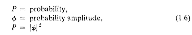
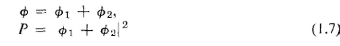
(2) When an event can occur in several alternative ways, the probability ampli-
tude for the event is the sum of the probability amplitudes for each way
considered separately. There is interference:
 i
i
(3) If an experiment is performed which is capable of determining whether one or
another alternative is actually taken, the probability of the event is the sum
of the probabilities for each alternative. The interference is lost:
One might still like to ask: "How does it work? What is the machinery behind
the law?" No one has found any machinery behind the law. No one can "explain"
any more than we have just "explained." No one will give you any deeper repre-
sentation of the situation. We have no ideas about a more basic mechanism from
which these results can be deduced.
We would like to emphasize a very important difference between classical and
quantum mechanics. We have been talking about the probability that an electron
will arrive in a given circumstance. We have implied that in our experimental
arrangement (or even in the best possible one) it would be impossible to predict
exactly what would happen. We can only predict the odds! This would mean, if
it were true, that physics has given up on the problem of trying to predict exactly
what will happen in a definite circumstance. Yes! physics has given up. We do
not know how to predict what would happen in a given circumstance, and we believe
now that it is impossible—that the only thing that can be predicted is the prob-
ability of different events. It must be recognized that this is a retrenchment in our
earlier ideal of understanding nature. It may be a backward step, but no one
has seen a way to avoid it.
We make now a few remarks on a suggestion that has sometimes been made
to try to avoid the description we have given: "Perhaps the electron has some kind
of internal works—some inner variables—that we do not yet know about. Perhaps
that is why we cannot predict what will happen. If we could look more closely at
the electron, we could be able to tell where it would end up." So far as we know,
that is impossible. We would still be in difficulty. Suppose we were to assume that
inside the electron there is some kind of machinery thai determines where it is
going to end up. That machine must also determine which hole it is going to go
through on its way. But we must not forget that what is inside the election should
not be dependent on what we do, and in particular upon whether we open or close
one of the holes. So if an electron, before it starts, has already made up its mind
(a) which hole it is going to use, and (b) where it is going to land, we should find
P1 for those electrons that have chosen-hole 1, P2 for those thai have chosen hole
2, and necessarily the sum P1 + P2 for those that arrive through the two holes.
There seems to be no way around this. But we have verified experimentally that
that is not the case. And no one has figured a way out of this puzzle. So at the
1-10
present time we must limit ourselves to computing probabilities. We say "at the
present time," but we suspect very strongly that it is something that will be with
us forever—that it is impossible to beat that puzzle—that this is the way nature
really is.
1-8 The uncertainty principle
This is the way Heisenberg stated the uncertainty principle originally: If you
make the measurement on any object, and you can determine the x-component of
its momentum with an uncertainty delta p, you cannot, at the same time, know its
x-position more accurately than delta x = h / delta p, where h is a definite fixed number
given by nature. It is called "Planck's constant," and is approximately 6.63 x
10-34 joule-seconds. The uncertainties in the position and momentum of a
particle at any instant must have their product greater than Planck's constant.
This is a special case of the uncertainty principle that was stated above more
generally. The more general statement was that one cannot design equipment in
any way to determine which of two alternatives is taken, without, at the same
time, destroying the pattern of interference.
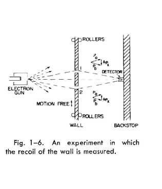
Let us show for one particular case that the kind of relation given by Heisen-
berg must be true in order to keep from getting into trouble. We imagine a modifi-
cation of the experiment of Fig. 1-3, in which the wall with the holes consists of a
plate mounted on rollers so that it can move freely up and down (in the x-direction),
as shown in Fig. 1-6. By watching the motion of the plate carefully we can try to
tell which hole an electron goes through. Imagine what happens when the detector
is placed at x = 0. We would expect that an electron which passes through hole 1
must be deflected downward by the plate to reach the detector. Since the vertical
component of the electron momentum is changed, the plate must recoil with an
equal momentum in the opposite direction. The plate will get an upward kick.
If the electron goes through the lower hole, the plate should feel a downward kick.
It is clear that for every position of the detector, the momentum received by the
plate will have a different value for a traversal via hole 1 than for a traversal via
hole 2. So! Without disturbing the electrons at all, but just by watching the plate,
we can tell which path the electron used.
Now in order to do this it is necessary to know what the momentum of the
screen is, before the electron goes through. So when we measure the momentum
after the electron goes by, we can figure out how much the plate's momentum has
changed. But remember, according to the uncertainty principle we cannot at the
same time know the position of the plate with an arbitrary accuracy. But if we do
not know exactly where the plate is, we cannot say precisely where the two holes are.
They will be in a different place for every electron that goes through. This means
that the center of our interference pattern will have a different location for each
electron. The wiggles of the interference pattern will be smeared out. We shall show
quantitatively in the next chapter that if we determine the momentum of the plate
sufficiently accurately to determine from the recoil measurement which hole was
used, then the uncertainty in the x-position of the plate will, according to the un-
certainty principle, be enough to shift the pattern observed at the detector up and
down in the x-direction about the distance from a maximum to its nearest minimum.
Such a random shift is just enough to smear out the pattern so that no interference
is observed.
The uncertainty principle "protects" quantum mechanics. Heisenberg recog-
nized that if it were possible to measure the momentum and the position simultane-
ously with a greater accuracy, the quantum mechanics would collapse. So he
proposed that it must be impossible. Then people sat down and tried to figure out
ways of doing it, and nobody could figure out a way to measure the position and
the momentum of anything—a screen, an electron, a billiard ball, anything—with
any greater accuracy. Quantum mechanics maintains its perilous but still correct
existence.
1-11